Scientific Software Development Course
This wiki page is about part I of SciNet's Scientific Computing course, given in 2011
Information about part II given in 2012 can be found on the page Numerical Tools for Physical Scientists (course)
Information on part III given in 2012 can be found on the page High Performance Scientific Computing
The 2013 Scientific Computing Course page is here.
Syllabus
The first of SciNet's for-credit courses (Phys 2109 modular course credit / Ast 3100 mini-course credit) will started in November, with the first lecture held in SciNet's conference room, but the subsequent lectures moved to the Astronomy building (see below). Dates are Nov 4, 11, 18, and 25th, 9:30-11:30am.
The goal of the first course is to have students learn the basics of best practice for writing maintainable, modular scientific programs. At the end of minicourse I, "Scientific Software Development", students arriving with fairly modest scientific programming knowledge will leave being able to:
- Do basic software development in a linux-like environment
- Write a modular scientific program in C
- Read and write Makefiles for building large pieces of software
- Be able to install simple libraries on their systems
- Use git for basic version control for software development (or paper writing)
- Use Python for basic visualization and data manipulation
- debug C programs with gdb/ddd
- write simple C++ and Python programs.
- use gprof or python profiling to find performance "hot spots"
The course will require 4-6 hours each week spent on reading and homework.
Required Software
Each lecture will have a hands-on component; students are strongly encouraged to bring laptops. (Contact us if this will be a problem). Windows, Mac, or Linux laptops are all fine, but some software will have to be installed *before* the first lecture:
On windows laptops only, Cygwin ( http://www.cygwin.com/) will have to be installed ; ensure that development tools (gcc/g++/gfortran, gdb), git, and the X environment (Xorg) is installed.
On Mac laptops, ensure that the development tools (Xcode) is installed.
On Linux, ensure that packages for the gcc compiler suite (gcc/g++/gfortran), gdb, and git are installed
On all platforms, the Enthought python distribution ( http://www.enthought.com/products/edudownload.php ) must be installed.
Students who aren't already comfortable with working in a shell / terminal environment should work through at least the first three 10-minute lectures at http://software-carpentry.org/4_0/shell/ .
Course outline
The classes will cover the material as follows; homework will be due by email at Thursday noon on the day before the following class.
Week 1 - Intro to software developemnt: basics of C, make, git. HW1: modular, multifile programming and make.
Week 2 - Simple parabolic PDEs; modular programming, refactoring, and testing. Simple visualization using python. HW2: Refactoring, testing, and debugging a simple PDE solver
Week 3 - Structures in C; simple ODE solvers and interpolation. HW3: tracer particle evolution
Week 4 - Going further with C++ and Python; profiling HW4: "porting" tracer particle evolution to C++
Evaluation
Evaluation will be based entirely on the four home works, with equal weighting given to each.
Location
First Lecture: SciNet offices at 256 McCaul, 2nd Floor.
Because of the higher than expected turn-up of students, the remaining three lectures of part 1 of SciNet's scientific computing course will be held at:
   Astronomy and Astrophysics Building
   50 St. George Street
   Room AB 107
   Same time and date: Friday 9:30 - 11:30.
Office Hours
The instructors will have office hours on Monday and Wednesday afternoons, 3pm-4pm, starting the week of the first class.
Location: SciNet offices at 256 McCaul, 2nd Floor.
- Mon, Oct 31, 3pm
- Wed, Nov 2, 3pm
- Mon, Nov 7, 3pm
- Wed, Nov 9, 3pm
- Mon, Nov 14, 3pm
- Wed, Nov 16, 3pm
- Mon, Nov 21, 3pm
- Wed, Nov 23, 3pm
- Mon, Nov 28, 3pm
- Wed, Nov 30, 3pm
Lectures
Lecture 1 (slides and video)
Intro to C, make and version control 
Slides
Recording
Lecture 2 (slides)
Python, modular programming, course project, diffusion PDE, debugging, testing
(Recording unfortunately crashed)
Slides
Lecture 3 (slides and recordings)
Structs in C, ODEs, Linking libraries
recording - part 1
recording - part 2
Slides
Lecture 4 (slides and video)
Part 1 - Debugging Slides
Part 2 - C++ Slides
Lecture - Video (large: 312MB)
Lecture - Video (small: 237MB)
Homeworks
Homework 1
We’ve learned programming in basic C, use of make and Makefiles to build projects, and local use of git for version control. In this first assignment, you’ll use these to make a multi-file C program, built with make, which computes and outputs a data file.
Start a new git repository, and begin writing a C program which gets an array size and a standard deviation from user input, allocates a 2d array, and stores a 2d Gaussian with a maximum at the centre of the array and with a standard deviation (in units of grid points in that array). The program then outputs that array to a text file, frees the array, and exits. The 2d array creation/freeing routines should be in one file (with an associated header file), the gaussian calculation be in another (ditto), and the output routine be in a third, with the main program calling each of these. The package should come with a Makefile which lets make build the software. (Note that you can start with everything in one file, and with hardcoded values for sizes and standard deviation and static array, and then refactor things into multiple files and add the “features” of user input and allocated arrays once the simplest part is working.)
The output text file should contain just the data in text format, with a row of the file corresponding to a row of the array and with whitespace between the numbers. You can include comments in the text file if you like, on lines that begin with the “#” character.
As a test, you should be able to use the ipython executable that came with your enthought python distribution to read your data and plot it. If your data file is named ‘data.txt’, running the following from the terminal:
$ ipython -pylab

In [1]: data = numpy.genfromtxt('data.txt')

In [2]: contour(data)
Should give you a nice contour plot of a 2-dimensional gaussian.
You will hand in your source code and the git log file of all your commits (and you will commit regularly!) by email by next Thursday at noon, so we can review the assignments and talk about any commonly occuring issues in Friday’s class. Email the files to rzon@scinet.utoronto.ca and ljdursi@scinet.utoronto.ca.
Homework 2
Today, we talked about modular programming and testing, and the project we’ll be working on for the next three weeks. This homework will start advancing on that project by working on the “legacy” code given to us by our prof, and whipping it into shape before we start adding new physics.
If you haven’t already, create a git repository that contains the source code ( diffuse2.c) and any related files (By the way, a decent Git cheatsheet can be found at the link below. Since you’re doing all local work, you can ignore the bits about “update and publish”, and “merge and release”: http://www.git-tower.com/files/cheatsheet/Git_Cheat_Sheet_grey.pdf )
For next Thursday, you’ll have refactored this into some sensible structure, with multiple files, and a Makefile. You’ll at least have factored out the main evolution code (which implements the diffusion operator on the 2d grid), and probably the array stuff, plotting stuff, and theory stuff as well. This should go pretty quickly, as it’s similar to last week’s work, and we’ll probably get a good start on it in class.
You’ll then design two tests for the evolution code, and have a separate make target which compiles the diffusion tests, such that on running that executable, one would find if the diffusion operator passed the tests or not. However, you do not have to implement the tests, only describe them in comment lines.
Next, you’ll read up on interpolation and ODEs (the references can be found below) and write the interface and stub implementation for an interpolation routine which, when given a 2d array of values and a floating-point (x,y) pair in grid coordinates on the grid, will calculate an interpolated value of the field at that point. There’s a number of interpolations which could make sense; just document what you’ve done. If the coordinate pair is out of bounds, return an error code. Design at least two tests routines for this interpolation code as well, with a separate make target for the interpolation test. Again, you do not have to implement the tests.
Finally, as a start to get the legacy code up and fully running with the plotting package that it was supposed to work with, install pgplot: http://www.astro.caltech.edu/~tjp/pgplot/ . The installation instructions are a bit odd but clear. We will get the final linking to diffuse2 done in class.
The marking scheme will be 20% git log, 20% Makefile, 20% refactoring, 30% tests, and 10% getting pgplot to work. Office hours will again be Mon and Wed, but this time both will be held by Ramses. You can always email us with questions.
You will hand in your source code, and the git log file of all your commits by email by next Thursday at noon, so we can review the assignments and talk about any commonly occuring issues in Friday’s class. Email the files to rzon@scinet.utoronto.ca and ljdursi@scinet.utoronto.ca.
Homework 3
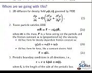
In this homework, we are going to implement the class project of a tracer particle coupled to a diffusion equation. The full specification of the physical problem is here.
In contrast to what was stated in class, given the time constraints, you are not required to finish the interpolation routine yourself. Get the solution to the interpolation and the interpolation test here.
And for those of you who did not finish the tracer particle implementation last friday, here is a sample code to start with. Note that this contains the theoretical predction for the constant diffusion case, in which case the equations are solvable. Comparison with the theoretical prediction can be a guide to determine what reasonable values for the time step are.
The homework, then, consists of the following two tasks:
1. Rewrite either from your own implementation of the tracer particle that you wrote in class, or this implementation, to work with a given density field such that alpha0 -> alpha(rho(x)) = alpha0(1 + a rho(x)) with a=15 (use the interpolation routine).
2. Start a new git project (or git branch from the diffusion code, if you know how to). For this new project, you are to implement the linked diffusion and the tracer particle evolution. In every time step, you update both the tracer particle and the density field, and you feed the density field back to the tracer particle to set its alpha value. For simplicity, you can use the same time step for both the diffusion and the tracer particle.
The marking scheme will be 20% git log, 20% Makefile and 60% implementation, equally divided over these two projects. Office hours will again on Wed, held by Jonathan. You can always email us with questions.
You will hand in your source code, makefiles and the git log file of all your commits by email by next Thursday at 8pm (note the extended time compare to the usual due time). Email the files, preferably zipped or tarred, to rzon@scinet.utoronto.ca and ljdursi@scinet.utoronto.ca.
Homework 4
In this homework, you are to port your C project of a tracer particle coupled to a diffusion equation to C++. The point is not to rewrite the low level parts, but to encapsulate the many parts that the project now contains in an object oriented fashion.
Your aim should be to have classes Diffusion, Tracer and Parameters (at the least), such that the following main function would work (after appropriate header files are included, of course): <source lang="cpp"> int main() {
   Parameters param;
   param.read();
   Diffusion part1;
   Tracer part2;
   part1.parameters(param);
   part2.parameters(param);
   part1.print();
   part2.print();
   for (int step = 0; step < param.nsteps; step++) {
       part1.couple(part2);
       part2.couple(part1);
       part1.compute();
       part2.compute();
       part1.evolve();
       part2.evolve();
       part1.print();
       part2.print();
   }
   return 0;
} </source> Note that this suggest that all parameters are taken together into one class Parameters, and that Tracer and Diffusion have the same interface. Make the latter happen by (publically) deriving both from the following class: <source lang="cpp"> class Parameters; class Diffusion; class Tracer; class DynamicSystem {
 public:
   virtual void parameters(Parameters& p) = 0;
   virtual void print() = 0;
   virtual void compute() = 0;
   virtual void evolve() = 0;
   virtual void couple(Diffusion& d) = 0;
   virtual void couple(Tracer& t) = 0;
   virtual ~DynamicSystem() {}
}; </source> A few other pointers:
- The " = 0;" causes these member functions to be undefined, and in that way you are forced to define them in derived classes (or the linker will shout at you). Such uninitialized functions are called 'pure virtual', and the class in called an Abstract Base Class (or ABC). For technical reasons, the destructor is never really pure virtual.
- Compilation of C++ code should be done with g++ instead of gcc, while the make command uses whatever is in the CXX variable (instead of CC). In addition, make's implicit rules for compiling C++ code use the CXXFLAGS variable instead of CFLAGS.
- Typical extensions for C++ programs are .cc, .cpp or .C (these are recognized by make's implicit rules)
- Typical extensions for C++ header files are .h, .hh, .hpp or .H
- Programs compiled with g++ typically have to be linked with g++ as well.
The marking scheme will be 20% each for the 1) git log, 2) Makefile and 3) Tracer class implementation 4) Diffusion class implementation, 5) rest of the code. Office hours will again be on Mon and Wed. You can always email us with questions.
You will hand in your source code, and the git log file of all your commits by email by next Thursday at noon. Email the files to rzon@scinet.utoronto.ca and ljdursi@scinet.utoronto.ca.
Links
Unix
- Cygwin: http://www.cygwin.com
- Intro to unix shell from software carpentry: http://software-carpentry.org/4_0/shell
C
- C preprocessor: http://www.cprogramming.com/tutorial/cpreprocessor.html
C++
Git
- Git cheat sheet from Git Tower: http://www.git-tower.com/files/cheatsheet/Git_Cheat_Sheet_grey.pdf
Python
- Enthought python distribution: http://www.enthought.com/products/edudownload.php
- Intro to python from software carpentry: http://software-carpentry.org/4_0/python
- Tutorial on matplotlib: http://conference.scipy.org/scipy2011/tutorials.php#jonathan
PGPLOT
- Pgplot plotting library: http://www.astro.caltech.edu/~tjp/pgplot
Interpolation (2D)
- Interpolation in Numerical Recipes for C: http://apps.nrbook.com/c/index.html Pages 123-128
- Wikipedia pages on Bilinear Interpolation and Bicubic Interpolation are not bad either.
ODEs
- Integrators for particle based ODEs (i.e. molecular dynamics): http://www.chem.utoronto.ca/~rzon/simcourse/partmd.pdf.
Focus on 4.1.4 - 4.1.6 for practical aspects. - Numerical algorithm to solve ODEs (General) in Numerical Recipes for C: http://apps.nrbook.com/c/index.html Chapter 16