Scientific Computing Course
This wiki page concerns the 2013 installment of SciNet's Scientific Computing course. Material from the previous installment can be found on Scientific Software Development Course, Numerical Tools for Physical Scientists (course), and High Performance Scientific Computing
Syllabus
About the course
- Whole-term graduate course
- Prerequisite: basic C, C++ or Fortran experience.
- Will use `C++ light' and Python
- Topics include: Scientific computing and programming skills, Parallel programming, and Hybrid programming.
There are three parts to this course:
- Scientific Software Development: Jan/Feb 2013
python, C++, git, make, modular programming, debugging - Numerical Tools for Physical Scientists: Feb/Mar 2013
modelling, floating point, Monte Carlo, ODE, linear algebra,fft - High Performance Scientific Computing: Mar/Apr 2013
openmp, mpi and hybrid programming
Each part consists of eight one-hour lectures, two per week.
These can be taken separately by astrophysics graduate students at the University of Toronto as mini-courses, and by physics graduate students at the University of Toronto as modular courses.
The first two parts count towards the SciNet Certificate in Scientific Computing, while the third part can count towards the SciNet HPC Certificate. For more info about the SciNet Certificates, see http://www.scinethpc.ca/2012/12/scinet-hpc-certificate-program.
Location and Times
SciNet HeadQuarters
256 McCaul Street, Toronto, ON
Room 229 (Conference Room)
Tuesdays 11:00 am - 12:00 noon
Thursdays 11:00 am - 12:00 noon
Instructors and office hours
- Ramses van Zon - 256 McCaul Street, Rm 228 - Mondays 3-4pm
- L. Jonathan Dursi - 256 McCaul Street, Rm 216 - Wednesdays 3-4pm
Grading scheme
Attendence to lectures.
Four home work sets (i.e., one per week), to be returned by email by 9:00 am the next Thursday.
Sign up
Sign up for this graduate course goes through SciNet's course website.
The direct link is https://support.scinet.utoronto.ca/courses/?q=node/99.
If you do not have a SciNet account but wish to register for this course, please email support@scinet.utoronto.ca .
Sign up is closed.
Part 1: Scientific Software Development
Prerequisites
Some programming experience. Some unix prompt experience.
Software that you'll need:
A unix-like environment with the GNU compiler suite (e.g. Cygwin), and Python 2, IPython, Numpy, SciPy and Matplotlib (which you all get if you use the Enthought distribution) installed on your laptop. Links are given at the bottom of this page.
Dates
January 15, 17, 22, 24, 29, and 31, 2013
February 5 and 7, 2013
Topics (with lecture slides and recordings)
Lecture 1: C++ introduction
Lecture 2: More C++, build and version control

- Guest lecturer: Michael Nolta (CITA) for the git portion of the lecture.
- C++ and Make slides / C++ and Make video recording / Git slides / Homework assigment 1
Lecture 3: Python and visualization
Lecture 4: Modular programming, refactoring, testing
Lecture 5: Object oriented programming
Lecture 6: ODE, interpolation
Lecture 7: Development tools: debugging and profiling
Lecture 8: Objects in Python, linking C++ and Python
Homework assignments
HW1
Multi-file C++ program to create a data file
We’ve learned programming in basic C++, use of make and Makefiles to build projects, and local use of git for version control. In this first assignment, you’ll use these to make a multi-file C++ program, built with make, which computes and outputs a data file.
- Start a git repository, and begin writing a C++ program to
- Get an array size and a standard deviation from user input,
- Allocate a 2d array (use the code given in lecture 2),
- Store a 2d Gaussian with a maximum at the centre of the array and given standard deviation (in units of grid points),
- Output that array to a text file,
- Free the array, and exit.
- The output text file should contain just the data in text format, with a row of the file corresponding to a row of the array and with whitespace between the numbers.
- The 2d array creation/freeing routines should be in one file (with an associated header file), the gaussian calculation be in another (ditto), and the output routine be in a third, with the main program calling each of these.
- Use a makefile to build your code (add it to the repository).
- You can start with everything in one file, with hardcoded values for sizes and standard deviation and a static array, then refactor things into multiple files, adding the other features.
- As a test, use the ipython executable that came with your Enthought python distribution to read your data and plot it.
If your data file is named ‘data.txt’, running the following:
$ ipython --pylab
In [1]: data = numpy.genfromtxt('data.txt')
In [2]: contour(data)
should give a nice contour plot of a 2-dimensional gaussian.
- Email in your source code, makefile and the "git log" output of all your commits by email by at 9:00 am Thursday Jan 24th, 2013. Please zip or tar these files together as one attachment, with a file name that includes your name and "HW1".
HW2
Refactor legacy code to a modular project with unit tests
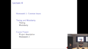
In class, today, we talked about modular programming and testing, and the project we’ll be working on for the next three weeks. This homework will start advancing on that project by working on the “legacy” code given to us by our supervisor (diffuse.cc), with a corresponding python plotting script (plotdata.py), and whipping it into shape before we start adding new physics.
- Start a git repository for this project, and add the two files.
- Create a Makefile and add it to the repository.
- Since we have no tests, run the program with console output redirected to a file:
$ diffuse > original-output.txt
It turns out the code has a bug that can make the output different when the same code is run again, which obviously would not be good for a baseline test. Replace 'float error;' by 'float error=0.0;' to fix this.
- Also save the two .npy output files, e.g. to original-data.npy and original-theory.npy. The triplet of files (original-output.txt, original-data.npy and original-theory.npy) serve as a baseline integrated test (add these to repository).
- Then write a 'test' target in your makefile that:
- Runs 'diffuse' with output to a new file.
- Compares the file with the baseline test file, and compare the .npy files.
- (hint: the unix command diff or cmp can compare files).
- First refactoring: Move the global variables into the main routine.
- Chorus: Test your modified code, and commit.
- Second refactoring: Extract a diffusion operator routine, that gets called from main.
- Chorus
- Create a .cc/.h module for the diffusion operator.
- Chorus
- Add two tests for the diffusion operator: for a constant and for a linear input field (rho[i][j]=a*i+b*j). Add these to the test target in the makefile.
- Chorus
- More refactoring: Extract three more .cc/.h modules:
- for output (should not contain hardcoded filenames)
- computation of the theory
- and for the array allocation stuff.
- Chorus
- Describe, but don't implement in the .h and .cc, what would be appropriate unit tests for these three modules.
Email in your source code and the git log file of all your commits as a .zip or .tar file by email to rzon@scinethpc.ca and ljdursi@scinethpc.ca by 9:00 am on Thursday January 31, 2013.
HW3
This week, we learned about object oriented programming, which fits nicely within the modular programming idea. In this homework, we are going to use some of it to restructure our code and get it ready to add the tracer particle, the goal of the course project.
The goal will be to have an instance of a Diffusion class, as well as an instance of Tracer, which for now will be a free particle moving as (x(t),y(t)) = (x(0) + vx t, y(0) + vy t), without any coupling yet (we will handle this next week).
To be more specific:
- Clean up your code, using the feedback from your HW2 grading, such that the modules are as independent as possible.
- If you have not done so yet, add comments to the header files of your modules to explain exactly what each function does (without going into implementation details), what its arguments mean and what it returns (unless it's a void function, of course).
- Objectify the main routine, by creating a class Diffusion.
- Put this class in its own module (declaration in .h, implementation in .cc). For instance, the declaration could be
// diffusion.h
#ifndef DIFFUSIONH
#define DIFFUSIONH
#include <fstream>
class Diffusion {
  public:
    Diffusion(float x1, float x2, float D, int numPoints);
    void init(float a0, float sigma0); // set initial field
    void timeStep(float dt);           // solve diff. equation over dt
    void toFile(std::ofstream& f);     // write to file (binary,no npyheader)
    void toScreen();                   // report a line to screen
    float getRho(int i, int j);        // get a value of the field
    ~Diffusion();
  private:
    float*** rho;
    ...
};
#endif
(this is not supposed to be prescriptive.)
- In the implementation file you'd have things like
// diffusion.cc
#include "diffusion.h"
...
void Diffusion::timeStep(float dt)
{
   // code for the timeStep ...
}
...
(note the inclusion of the module's header file on the top of the implementation, so the class is declared).
- Let int main() have the same functionality as before, but now by defining the parameters of the run, creating an object of this class, setting up file streams, and taking time steps and writing out by using calls to member functions of this object.
- Additionally, write a class Tracer which for now implements a free particle in 2d. Something like:
class Tracer {
  public:
    Tracer(float x1, float x2);
    void init(float x0, float y0, float vx, float vy);
    void timeStep(float dt);           // solve diff. equation over dt
    void toFile(std::ofstream& f);     // write to file (binary,no npyheader)
    void toScreen();                   // report a line to screen
    ~Tracer();
  private:
    ...
};
- The timeStep implementation can in this case use the infamous forward Euler integration scheme, because it happens to be exact here.
- When it comes to output to a npy file, let's view the the data of the tracer particle at one point in time as a 2x2 matrix [[x,y],[vx,vy]], so we can use much of the npy output code that we used for the diffusion field, which was a (numPoints+2)x(numPoints+2) matrix.
- This class too should be its own module (Often, "one class, one module" is a good paradigm, though occasionally you'll have closely related classes).
- Add some code to int main to have the Tracer particle evolve at the same time as the diffusion field (although the two are completely uncoupled).
- Keep using git and make, run the tests that you have regularly to make sure your program still works.
Note that because we've now set up our program in a modular fashion, you can do different parts of this assignment in any order you want. For instance, to wrap your head around object oriented programming, you may like implementing the tracer particle first, so that your diffusion code stays intact. Or you might want to wait with commenting until the end if you think you'll have to change a module for this assignment.
Email in your source code and the git log file of all your commits as a .zip or .tar file by email to rzon@scinethpc.ca and ljdursi@scinethpc.ca by 3:00 pm on Friday February 8, 2013.
HW4
TBA
Part 2: Numerical Tools for Physical Scientists
Prerequisites
Part 1 or solid c++ programming skills, including make and unix/linux prompt experience.
Software that you'll need
A unix-like environment with the GNU compiler suite (e.g. Cygwin), and Python (Enthought) installed on your laptop.
Dates
February 12, 14, 26, and 28, 2013
March 5, 7, 12, and 14, 2013
Topics
Lecture 9 Numerics
Lecture 10 Random numbers
Lecture 11 Numerical integration and ODEs
Lecture 12 Molecular Dynamics
Lecture 13 Linear Algebra part I
Lecture 14 Linear Algebra part II and PDEs
Lecture 15 Fast Fourier Transform
Lecture 16 FFT for real and multidimensional data
Part 3: High Performance Scientific Computing
Prerequisites
Part 1 or good c++ programming skills, including make and unix/linux prompt experience.
Software that you'll need
You will need to bring a laptop with a ssh facility. Hands-on parts will be done on SciNet's GPC cluster.
For those who don't have a SciNet account yet, the instructions can be found at http://wiki.scinethpc.ca/wiki/index.php/Essentials\#Accounts
Dates
March 19, 21, 26, and 28, 2013
April 2, 4, 9, and 11, 2013
Topics
Lecture 17 Intro to Parallel Computing
Lecture 18 Parallel Computing Paradigms
Lecture 19 Shared Memory Programming with OpenMP, part 1
Lecture 20 Shared Memory Programming with OpenMP part 2
Lecture 21 Distributed Parallel Programming with MPI, part 1
Lecture 22 Distributed Parallel Programming with MPI, part 2
Lecture 23 Distributed Parallel Programming with MPI, part 3
Lecture 24 Hybrid OpenMPI+MPI Programming
Links
Unix
- Cygwin: http://www.cygwin.com
- Linux Command Line: A Primer (June 2012) Slides, Files
- Intro to unix shell from software carpentry: http://software-carpentry.org/4_0/shell
C/C++
- One-Day Scientific C++ Class at SciNet
- C++ library reference: http://www.cplusplus.com/reference
- C preprocessor: http://www.cprogramming.com/tutorial/cpreprocessor.html
- Boost: http://www.boost.org
- Boost Python tutorial: http://www.boost.org/doc/libs/1_53_0/libs/python/doc/tutorial/doc/html/index.html
Git
- Git: http://git-scm.com
- Version Control: Video/ Slides
- Git cheat sheet from Git Tower: http://www.git-tower.com/files/cheatsheet/Git_Cheat_Sheet_grey.pdf
Python
- Python: http://www.python.org
- IPython: http://ipython.org
- Matplotlib: http://www.matplotlib.org
- Enthought python distribution: http://www.enthought.com/products/edudownload.php
(this gives you numpy, matplotlib and ipython all installed in one fell swoop)
- Intro to python from software carpentry: http://software-carpentry.org/4_0/python
- Tutorial on matplotlib: http://conference.scipy.org/scipy2011/tutorials.php#jonathan
- Npy file format: https://github.com/numpy/numpy/blob/master/doc/neps/npy-format.txt
- Boost Python tutorial: http://www.boost.org/doc/libs/1_53_0/libs/python/doc/tutorial/doc/html/index.html
ODEs
- Integrators for particle based ODEs (i.e. molecular dynamics): http://www.chem.utoronto.ca/~rzon/simcourse/partmd.pdf.
Focus on 4.1.4 - 4.1.6 for practical aspects. - Numerical algorithm to solve ODEs (General) in Numerical Recipes for C: http://apps.nrbook.com/c/index.html Chapter 16
Interpolation (2D)
- Interpolation in Numerical Recipes for C: http://apps.nrbook.com/c/index.html Pages 123-128
- Wikipedia pages on Bilinear Interpolation and Bicubic Interpolation are not bad either.


